SVMの実装
数値例のデータセットの読み込み
[1]:
%matplotlib inline
import numpy as np
import pandas as pd
import matplotlib.pyplot as plt
[2]:
df = pd.read_csv('sample_perceptron.csv')
[3]:
df.head(3)
[3]:
| t | x0 | x1 | x2 | |
|---|---|---|---|---|
| 0 | 1 | 1 | -1.235948 | -2.599843 |
| 1 | 1 | 1 | -2.021262 | -0.759107 |
| 2 | 1 | 1 | -1.132442 | -3.977278 |
[94]:
t = df[['t']].values
X = df.iloc[:, 1:].values
プロット用に各カテゴリのデータも抽出しておきましょう。
[95]:
x_1 = df[df['t'] == 1].iloc[:, 2:].values
x_2 = df[df['t'] == -1].iloc[:, 2:].values
データの可視化
パラメータ\(w\)の調整に入る前に、現状どの程度の識別の結果が得られているのか確認できるような可視化の関数を作成しておきましょう。
パーセプトロンでは識別の境界線を入力が二次元の場合、以下のように定式化しています。
\(w_{1}x_{1} + w_{2}x_{2} + w{0} = 0\)
縦軸\(x2\)に関して整理すると以下のようになります。
\(x_{2} = - \dfrac{w_{1}x_{1} + w_{0}}{w_{2}}\)
[96]:
w = np.array([[0], [-1], [1]])
print(w)
[[ 0]
 [-1]
 [ 1]]
[97]:
def plot_result(w, x_1, x_2):

    x1 = np.linspace(-4, 4)
    x2 = - (w[1] * x1 + w[0]) / w[2]

    plt.plot(x1, x2, label='wx+b=0')
    plt.scatter(x_1[:, 0], x_1[:, 1], label='x1')
    plt.scatter(x_2[:, 0], x_2[:, 1], label='x2')
    plt.legend()
    plt.xlim([-5, 5])
    plt.ylim([-5, 5])
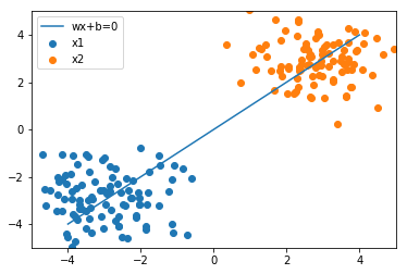
[98]:
plot_result(w, x_1, x_2)
損失関数
\(\mathcal{L} = \dfrac{1}{2} \alpha^{T}H \alpha - 1^{T}\alpha,\ H = (tt^{T}) \circ (XX^{T})\)
s.t. \(t^{T} \alpha = 0,\ -{\rm diag}(1)^{T} \alpha \leq 0\)
\(\displaystyle w = \sum_{n=1}^{N} \alpha_{n} t_{n} x_{n}\)
[143]:
N, M = X.shape
[144]:
N
[144]:
200
[101]:
T = np.dot(t, t.T)
[102]:
T.shape
[102]:
(200, 200)
[103]:
XX = np.dot(X, X.T)
[104]:
XX.shape
[104]:
(200, 200)
[105]:
H = T * XX
[106]:
from cvxopt import matrix, solvers
[118]:
q = matrix(-np.ones(N))
P = matrix(H)
G = matrix(np.diag(-np.ones(N)))
h = matrix(np.zeros(N))
A = matrix(t.T, tc='d')
b = matrix(0.0)
[119]:
sol = solvers.qp(P, q, G, h, A, b)
     pcost       dcost       gap    pres   dres
 0: -1.0309e+01 -1.6549e+01  5e+02  2e+01  2e+00
 1: -6.7867e+00 -1.2387e+00  4e+01  2e+00  2e-01
 2: -1.0048e-01 -2.2208e-01  5e-01  2e-02  1e-03
 3: -8.5655e-02 -1.4525e-01  8e-02  1e-03  8e-05
 4: -1.2179e-01 -1.3758e-01  2e-02  2e-04  1e-05
 5: -1.3355e-01 -1.3730e-01  4e-03  1e-05  9e-07
 6: -1.3705e-01 -1.3711e-01  6e-05  2e-07  1e-08
 7: -1.3711e-01 -1.3711e-01  6e-07  2e-09  1e-10
 8: -1.3711e-01 -1.3711e-01  6e-09  2e-11  1e-12
Optimal solution found.
[120]:
sol
[120]:
{'dual infeasibility': 1.2538396639065762e-12,
 'dual objective': -0.13711169851634578,
 'dual slack': 7.055007988875721e-10,
 'gap': 6.456624835283598e-09,
 'iterations': 8,
 'primal infeasibility': 1.6018880680528198e-11,
 'primal objective': -0.13711169231335898,
 'primal slack': 1.6159189474970968e-11,
 'relative gap': 4.7090257047717296e-08,
 's': <200x1 matrix, tc='d'>,
 'status': 'optimal',
 'x': <200x1 matrix, tc='d'>,
 'y': <1x1 matrix, tc='d'>,
 'z': <200x1 matrix, tc='d'>}
[128]:
alpha = np.array(sol['x'])
[137]:
w = np.zeros((1, 3))
for n in range(N):
    w += t[n] * alpha[n] * X[n]
[138]:
w
[138]:
array([[ 5.82438262e-17, -3.09349177e-01, -4.22523944e-01]])
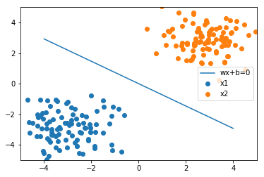
[142]:
plot_result(w.T, x_1, x_2)
[ ]: