パーセプトロンの実装
数学ノート
数値例用のデータセット作成
[1]:
%matplotlib inline
import numpy as np
import pandas as pd
import matplotlib.pyplot as plt
[2]:
# シードを固定して再現性の確保
np.random.seed(0)
[3]:
x1 = np.random.randn(100, 2)
x1 = x1 - 3
x2 = np.random.randn(100, 2)
x2 = x2 + 3
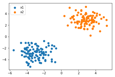
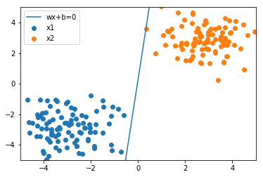
データはプロットして確認するとミスを防げます。
[4]:
plt.scatter(x1[:, 0], x1[:, 1], label='x1')
plt.scatter(x2[:, 0], x2[:, 1], label='x2')
plt.legend()
[4]:
<matplotlib.legend.Legend at 0x28dfa856a90>
教師データ作成
[5]:
# 1 0r -1 のラベルを付ける
t1 = [1] * len(x1)
t2 = [-1] * len(x2)
[6]:
# 縦向きに連結
x = np.r_[x1, x2]
t = np.r_[t1, t2]
[7]:
x.shape
[7]:
(200, 2)
[8]:
t.shape
[8]:
(200,)
CSVファイルにデータセットを保存
[9]:
# バイアス項も考慮して、すべてが1の列x0も追加
df = pd.DataFrame({
    'x0': [1] * len(x),
    'x1': x[:, 0],
    'x2': x[:, 1],
    't': t
})
[10]:
# 先頭3件
df.head(3)
[10]:
| t | x0 | x1 | x2 | |
|---|---|---|---|---|
| 0 | 1 | 1 | -1.235948 | -2.599843 |
| 1 | 1 | 1 | -2.021262 | -0.759107 |
| 2 | 1 | 1 | -1.132442 | -3.977278 |
[11]:
# 末尾3件
df.tail(3)
[11]:
| t | x0 | x1 | x2 | |
|---|---|---|---|---|
| 197 | -1 | 1 | 2.708163 | 2.238508 |
| 198 | -1 | 1 | 3.857924 | 4.141102 |
| 199 | -1 | 1 | 4.466579 | 3.852552 |
Pandasでは簡単にCSVファイルへ保存することができます。引数でindex_labelをFalseにしておかないと、一番左の行番号まで入ってしまうので注意です。
[12]:
df.to_csv('sample_perceptron.csv', index_label=False)
データの読み込み
今回は必要ありませんが、データの受け渡しがあった前提で読み込みも行いましょう。
[13]:
df = pd.read_csv('sample_perceptron.csv')
[14]:
df.head()
[14]:
| t | x0 | x1 | x2 | |
|---|---|---|---|---|
| 0 | 1 | 1 | -1.235948 | -2.599843 |
| 1 | 1 | 1 | -2.021262 | -0.759107 |
| 2 | 1 | 1 | -1.132442 | -3.977278 |
| 3 | 1 | 1 | -2.049912 | -3.151357 |
| 4 | 1 | 1 | -3.103219 | -2.589401 |
[15]:
t = df.iloc[:, 0].values
X = df.iloc[:, 1:].values
プロット用に各カテゴリのデータも抽出しておきましょう。
[16]:
x_1 = df[df['t'] == 1].iloc[:, 2:].values
x_2 = df[df['t'] == -1].iloc[:, 2:].values
データの可視化
パラメータ\(w\)の調整に入る前に、現状どの程度の識別の結果が得られているのか確認できるような可視化の関数を作成しておきましょう。
パーセプトロンでは識別の境界線を入力が二次元の場合、以下のように定式化しています。
\(w_{1}x_{1} + w_{2}x_{2} + w{0} = 0\)
縦軸\(x2\)に関して整理すると以下のようになります。
\(x_{2} = - \dfrac{w_{1}x_{1} + w_{0}}{w_{2}}\)
[17]:
w = np.array([[0], [-1], [1]])
print(w)
[[ 0]
 [-1]
 [ 1]]
[18]:
x1 = np.linspace(-4, 4)
x2 = - (w[1] * x1 + w[0]) / w[2]
[19]:
x1[:10]
[19]:
array([-4.        , -3.83673469, -3.67346939, -3.51020408, -3.34693878,
       -3.18367347, -3.02040816, -2.85714286, -2.69387755, -2.53061224])
[20]:
x2[:10]
[20]:
array([-4.        , -3.83673469, -3.67346939, -3.51020408, -3.34693878,
       -3.18367347, -3.02040816, -2.85714286, -2.69387755, -2.53061224])
[21]:
plt.plot(x1, x2, label='wx+b=0')
plt.scatter(x_1[:, 0], x_1[:, 1], label='x1')
plt.scatter(x_2[:, 0], x_2[:, 1], label='x2')
plt.legend()
# 最大値と最小値の領域も追加
plt.xlim([-5, 5])
plt.ylim([-5, 5])
[21]:
(-5, 5)
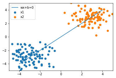
こちらのように可視化ができました。今の重みだと全然分類がうまくできていないことがわかります。そのため、パラメータを調整していくことで、うまく識別ができるかをこの後に確認していきましょう。
また、最後にプロットを行う関数にひとまとめにしておきましょう。
[22]:
def plot_result(w, x_1, x_2):

    x1 = np.linspace(-4, 4)
    x2 = - (w[1] * x1 + w[0]) / w[2]

    plt.plot(x1, x2, label='wx+b=0')
    plt.scatter(x_1[:, 0], x_1[:, 1], label='x1')
    plt.scatter(x_2[:, 0], x_2[:, 1], label='x2')
    plt.legend()
    plt.xlim([-5, 5])
    plt.ylim([-5, 5])
[23]:
plot_result(w, x_1, x_2)

損失関数の計算
まずは損失関数の定義から行いましょう。
ヒンジ損失関数
\(\displaystyle \mathcal{L} = \sum_{n=1}^{N} \max (0, -t_{n}y_{n})\)
ポイントとしては、各サンプルごとに計算できるようにしておきましょう。ここで気を付ける点として、\(x\)が数学上は縦向きのベクトルで扱いますが実装上はXの各行に格納されているため、横向きのベクトルになります。無理やり縦向きにしても良いのですが、\(x^{T}w\)のような計算のケースだと横向きのまま扱って、np.dot(x, w)としてしまう方が楽です。
[24]:
def hinge(t, x, w):
    y = np.dot(x, w)
    return max(0, -t * y)
関数の定義ができれば、まず動作するかの確認を行いましょう。
[25]:
x = X[0]
print(x)
[ 1. -1.23594765 -2.59984279]
[26]:
_t = t[0]
print(_t)
1
[27]:
hinge(_t, x, w)
[27]:
array([1.36389514])
このように動作できることを確認しました。
損失関数の勾配を計算
次は損失関数の勾配 \(\dfrac{\partial}{\partial w} \mathcal{L}\) を計算する関数を定義していきましょう。
[28]:
def grad_loss(t, X, w):

    # 勾配を格納するゼロベクトルを初期化
    grad = np.zeros((1, len(w)))

    for (_t, x) in zip(t, X):
        loss = hinge(_t, x, w)
        # 不正解の時は足し合わせる
        if loss > 0:
            grad += - _t * x

    return grad.T
損失関数の勾配も同様に確認していきます。
[29]:
grad = grad_loss(t, X, w)
print(grad)
[[  5.        ]
 [225.81531709]
 [332.56056004]]
最急降下法を実装
最急降下法に基づきパラメータを更新する関数 update を作成しましょう。alphaはハイパーパラメータとしてデフォルトの値を設定しておくと便利です。
\(w \leftarrow w - \alpha \dfrac{\partial}{\partial w} \mathcal{L}\)
[30]:
def update(w, grad, alpha=0.001):
    w = w - alpha * grad
    return w
パラメータ更新の様子を確認
まずは初期値を設定します。
[31]:
np.random.seed(100)
[32]:
w = np.array([[0], [-1], [1]])
print(w)
[[ 0]
 [-1]
 [ 1]]
[33]:
plot_result(w, x_1, x_2)

初期値では全然うまく分類できておらず、下記の3手順を繰り返しながらパラメータの更新を行っていきましょう。
損失関数の勾配を計算
パラメータのアップデート
結果の可視化
更新1回目
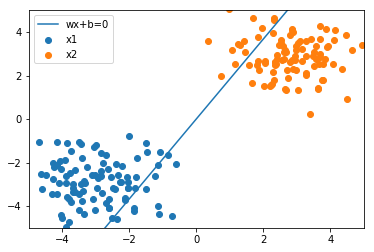
[34]:
grad = grad_loss(t, X, w)
w = update(w, grad)
print('grad:\n', grad)
print('w:\n', w)
plot_result(w, x_1, x_2)
grad:
 [[  5.        ]
 [225.81531709]
 [332.56056004]]
w:
 [[-0.005     ]
 [-1.22581532]
 [ 0.66743944]]
更新2回目
[35]:
grad = grad_loss(t, X, w)
w = update(w, grad)
print('grad:\n', grad)
print('w:\n', w)
plot_result(w, x_1, x_2)
grad:
 [[ 4.        ]
 [37.07200501]
 [94.28825842]]
w:
 [[-0.009     ]
 [-1.26288732]
 [ 0.57315118]]
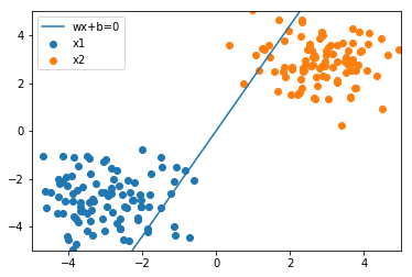
100回更新する
[36]:
for i in range(100):
    grad = grad_loss(t, X, w)
    w = update(w, grad)
[37]:
w
[37]:
array([[-0.039     ],
       [-1.34672437],
       [ 0.13553265]])
[38]:
grad
[38]:
array([[0.],
       [0.],
       [0.]])
[39]:
plot_result(w, x_1, x_2)
実際にパーセプトロンのアルゴリズムによって境界を決める識別線を求めることができました。
[ ]: